Are you a #1 team when it comes to document sharing? Learn these clever tricks to make your team excel… with Excel!
CONTEXT: You work with documents shared with a team. A same document is passed from one team member to the other.
GOAL: You want to enable the user inheriting of the Excel spreadsheet to (1) Understand at a glance the dependencies on the document; (2) Understand the logic of the calculations on the spreadsheet; (3) Be aware of the impact on the spreadsheet as a whole, should they modify any given cell.
USEFUL WHEN: (1) You are about to hand your Excel spreadsheet to a colleague, either because you are shifting mandates or because you are delegating work to to them or you need their input; (2) You are about to receive a spreadsheet from a colleague and he is not available to brief you on the details of its content; (3) You want to send a document to your boss or client to highlight the impact of a particular functionality or business decision on the cost of the project.
EXCEL CONCEPTS & FUNCTIONALITIES TO MASTER:
The following are the basics you need to complete the goal listed above. Simply follow the links if you need a refresher on the how-to portion of these functionalities.
1. Show formula (or, Clt + tilde ~) : The first thing you may want to do when you receive a document from someone is to make all formulas displayed so you may understand what is the result of a calculation and what is an arbitrary constant.
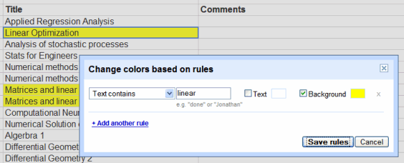
2. Find and select formulas (F5): To make it even more visible, you may want to highlight all the formulas in your spreadsheet with a color bucket. For instance, show me all the formulas in my spreadsheet highlighted in yellow. Simply hit the color bucket after you have found and selected the formulas. This may come in handy if you want to share a document with a co-worker as well.
3. Find and select constants (F5): Similarly, you may want to highlight constants, meaning number values that were manually entered by the user, and not calculated. You may use the color bucket tool after finding and selecting the constants, to make it easy to spot in your sheet. This may come in handy if you want to share a document with a co-worker as well.
4. Trace dependency (repeatedly): If you want to show a coworker the way modifying a specific cell will impact the entire worksheet, or if you want to make sure you will not affect anything when modifying data on someone’s Excel, you may trace dependencies repeatedly until the computer produces a sound indicating there are no more dependencies. This will create a network of arrows from one cell to another to show the dependencies to that cell.
5. Trace precedence (repeatedly): You may also want to visually show how the cell you are about to format is linked to other cells before it. You may use the trace precedence button repeatedly to do so.
6. Remove arrow: If you have used the trace dependency or trace precedence buttons, you will want to eventually clear the arrows. Use this button to do so.
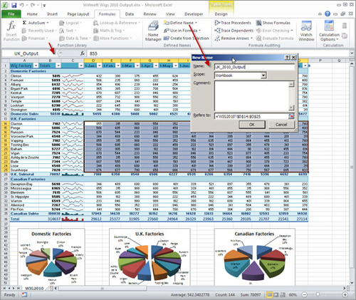
7. Name Range & Name box: This function is useful either to see the logic in a spreadsheet you’ve received (provided your colleague has entered name ranges) or to prepare your spreadsheet for your client, colleague or boss. You will use the name box on the left of the formula bar to assign a name to a cell, which will appear by name in every formula where the cell is used, as opposed to cryptic ”C5 * D9” formulas. This makes it easy for someone or even for yourself to change the values of variables in your data (ex. tax rates, commissions, price markups, etc.) if the data changes over time.
8. Convert portion of a table to a single name range (F3): If you are about to perform a series of operations (ex. median, average, etc.) on selected cells in a spreadsheet (ex. a table of rows and columns), you can give a name to the entire set of cells, and just refer to it when you write formulas, instead of having to select the cell ranges again and again.
9. Convert top row labels to name range: A quick way to generate name ranges is also to convert the labels on the top row of your table into name ranges. Then, whenever you apply a calculation to any given row, using the column range names, the formula automatically substitutes the row-specific information to your generic formula. In other words, it will seek the specific value for the cell listed under the generic column name. This makes it easier to perform ”conceptual” calculations and reduces the risk of mistakes when selecting cells manually. It also helps others understand the logic of your calculations.
10. Delete name range: If you notice a certain name range was never used or if you no longer want it to be available to users, you may delete it. Be aware the formulas associated to it will no longer work. To circumvent this issue, you may use special paste options to change your values from formulas into absolute values, prior to deleting a name range.
8. Display portion of the formula (F9): Lastly, this little trick will make your life easier when you are deciphering someone else’s spreadsheet (or reviewing your own), and feel that something is off in the numbers. It is possible for you to highlight a long formula and compute only a small sub-section of the big equation, to see if those numbers make sense. If you’re familiar with the ranges of the values (i.e. what they should roughly be equal to) within an equation, it may help you to quickly spot which portion of the formula is dysfunctional or inaccurate. This is an ”eye-ball” method to spot mistakes, but may be your best bet if you have long windy formulas with no name ranges.


